Apr 5, 2026 · 13 min read

Cosine Similarity vs Claude: What Happens When They Disagree

The problem with “similarity” is that it means different things depending on who you ask.

Ask an embedding model to score “I love you” against “I hate you”. The cosine similarity comes back at 78/100 — both are short declarations of intense emotion toward a person, sharing syntactic structure and training signal. The vectors end up close together even though the meanings are opposite.

Ask Claude the same question. It scores them at 15/100 and explains exactly why: “they express completely opposite feelings — love versus hate… the core emotional content is as different as two phrases can be.”

That gap is not a bug. It’s a window into how these two approaches to meaning actually work. I wanted to surface it directly, so I built a tool that shows both scores at once.

What embeddings actually are

An embedding model maps text to a point in a high-dimensional vector space — 768 dimensions for the model I’m using. The goal is for texts with similar meaning to end up nearby, and texts with different meanings to end up far apart.

“Nearby” is measured by cosine similarity: the cosine of the angle between two vectors. It ignores magnitude (how long the vectors are) and only cares about direction.

$\text{cosine\_similarity}(\mathbf{a}, \mathbf{b}) = \frac{\mathbf{a} \cdot \mathbf{b}}{\|\mathbf{a}\| \|\mathbf{b}\|} = \frac{\sum_{i=1}^{n} a_i b_i}{\sqrt{\sum_{i=1}^{n} a_i^2} \cdot \sqrt{\sum_{i=1}^{n} b_i^2}}$

Cosine similarity normalizes by magnitude, making the comparison purely directional — two texts about the same topic should point the same way in vector space regardless of length or phrasing. Dot product would conflate direction with magnitude, neither of which reliably encodes topical similarity on its own.

The deeper question is: what does the model learn to put near each other?

The answer goes back to the distributional hypothesis, articulated by the linguist J.R. Firth in 1957: “You shall know a word by the company it keeps.” ^{[Firth, J.R. (1957). “A synopsis of linguistic theory 1930-55.” Studies in Linguistic Analysis.]} Words that appear in similar contexts — surrounded by similar other words — tend to have similar meanings. Modern embedding models generalize this from words to full sentences and documents, trained on large-scale mixtures of supervised and unsupervised pairs (text, similar-text) using contrastive objectives: pull semantically similar pairs together, push dissimilar pairs apart.

This works remarkably well. It’s also why antonyms are a trap.

“The economy is growing” and “The economy is shrinking” appear in nearly identical contexts — financial news, economic forecasts, policy discussions. An embedding model trained on distributional statistics sees two texts that live in the same neighborhood. The vectors end up close. The model has no mechanism for “these are opposite claims” — it only knows they’re both things people say about economies. Cosine similarity measures topical proximity, not semantic agreement.

Claude is also a statistical model trained on text — it’s not doing symbolic reasoning or consulting a dictionary. But there are three meaningful architectural differences. First, it processes both texts jointly with full attention rather than compressing each into an independent fixed vector, so it can attend to the relationship between them. Second, it’s trained at scale on data that includes explicit reasoning about language — entailment, contradiction, natural language inference — so it has learned to produce outputs consistent with understanding antonymy and negation. Third, it generates its answer token by token, which allows something closer to deliberate comparison rather than a single forward pass to a fixed vector.

The result behaves like judgment even if the mechanism is still learned and statistical. Whether that constitutes “understanding” is a harder question — but behaviorally, it reliably catches what cosine similarity misses.

The model: nomic-embed-text-v1.5

The embedding model I’m using is nomic-embed-text-v1.5 (Nussbaum et al., 2024), which has two properties worth knowing about.

Matryoshka Representation Learning. The 768-dim vectors are structured so that the first n dimensions are themselves a valid embedding space for any n. You can truncate to 256 or 128 dimensions and the model still performs well — you trade a little accuracy for a lot of storage and compute savings. For 29 blog posts this doesn’t matter, but at scale it’s a meaningful design choice. The technique comes from Kusupati et al. (2022).

Prefix-aware encoding. The model uses instruction prefixes to distinguish retrieval from semantic similarity tasks — a pattern introduced by the E5 family of models (Wang et al., 2022). Corpus documents get "search_document: " prepended; queries get "search_query: ". This asymmetry lets the model optimize for what you actually care about: the document representation should be rich and general, the query representation should capture intent. Without prefixes, you’re leaving performance on the table.

prefix = "search_query: " if item.get("query") else "search_document: "
prefixed = [prefix + t for t in texts]

The architecture

There are two things to build: a tool that compares arbitrary text pairs, and semantic search over my blog. They share infrastructure — a Modal-hosted embedding endpoint.

I wrapped nomic-embed-text-v1.5 in a FastAPI ASGI app deployed on Modal with a /embed route for generating embeddings and a /project route that runs PCA to reduce the corpus to 2D for visualization:

@web_app.post("/embed")
def embed(item: dict) -> dict:
    from fastembed import TextEmbedding  # github.com/qdrant/fastembed
    model = TextEmbedding("nomic-ai/nomic-embed-text-v1.5")
    prefix = "search_query: " if item.get("query") else "search_document: "
    prefixed = [prefix + t for t in item.get("texts", [])]
    embeddings = list(model.embed(prefixed))
    return {"embeddings": [e.tolist() for e in embeddings]}

@web_app.post("/project")
def project(item: dict) -> dict:
    import numpy as np
    from sklearn.decomposition import PCA
    embeddings = np.array(item["embeddings"], dtype=np.float32)
    pca = PCA(n_components=2)
    coords = pca.fit_transform(embeddings)
    return {
        "coords": coords.tolist(),
        "mean": pca.mean_.tolist(),
        "components": pca.components_.tolist(),
    }

min_containers=1 keeps one container warm. For debounced search this matters — a 3-second cold start on every keystroke would be unusable.

Semantic search: build-time embeddings, browser-side similarity

For blog search, everything expensive happens at build time. A Node.js script reads all posts, strips markdown, calls Modal, and writes public/embeddings.json. At query time the user’s text goes through a Netlify function (to keep the Modal URL server-side), returns as a 768-dimensional vector, and gets scored against the pre-loaded corpus in the browser:

function cosineSim(a, b) {
  let dot = 0, na = 0, nb = 0;
  for (let i = 0; i < a.length; i++) {
    dot += a[i] * b[i];
    na += a[i] * a[i];
    nb += b[i] * b[i];
  }
  return dot / (Math.sqrt(na) * Math.sqrt(nb));
}

The conventional approach to semantic search involves a vector database — Pinecone, Weaviate, pgvector — that indexes embeddings and handles approximate nearest-neighbor queries at runtime. For a blog with 29 posts, that’s enormous infrastructure for a trivial problem.

Instead: no search index, no vector database, no runtime infrastructure beyond a single Netlify function call. The entire corpus — 29 posts × 768 floats × 4 bytes — is 400KB of JSON served as a static file. The browser fetches it once, holds it in memory, and runs exact cosine similarity against every post in milliseconds. At this scale, brute-force is the right algorithm.

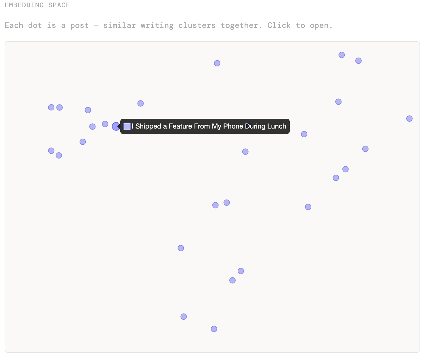
PCA projection of 29 blog posts into 2D embedding space

The scatter plot uses the PCA coordinates stored at build time. To project a new query point into the same 2D space, you apply the stored PCA transform — subtract the mean, multiply by the principal components. This is O(768 × 2) per query and runs instantly in the browser. PCA on 29 points in 768 dimensions won’t produce clean clusters — the structure is subtle — but topical proximity does emerge without any labels.

The dual-score tool: where it gets interesting

The Embedding Similarity tool runs both scores in sequence. Embeddings first (faster, since Modal is warm), then Claude with the cosine score passed as context:

// Step 1: embed both texts in parallel, compute cosine similarity
const [{ embedding: embA }, { embedding: embB }] = await Promise.all([...]);
const embeddingScore = Math.round(cosineSim(embA, embB) * 100);

// Step 2: Claude sees the embedding score and can address divergence
const compareRes = await fetch("/api/compare", {
  body: JSON.stringify({ textA, textB, embeddingScore }),
});

The prompt instructs Claude to explain divergences when they exceed 15 points. This turned out to be the most useful part of the output — not the scores themselves, but Claude’s reasoning about why a geometric measure and a language model are looking at the same pair of sentences differently.

Embedding score vs Claude's take on two sentences that diverge sharply

What the divergences reveal

Three patterns — and one non-divergence worth noting. Real scores from the live tool:

Pair	Embedding	Claude	Divergence
”I love you” / “I hate you”	78	15	63 pts
Legal clause / plain-English restatement	72	88	16 pts
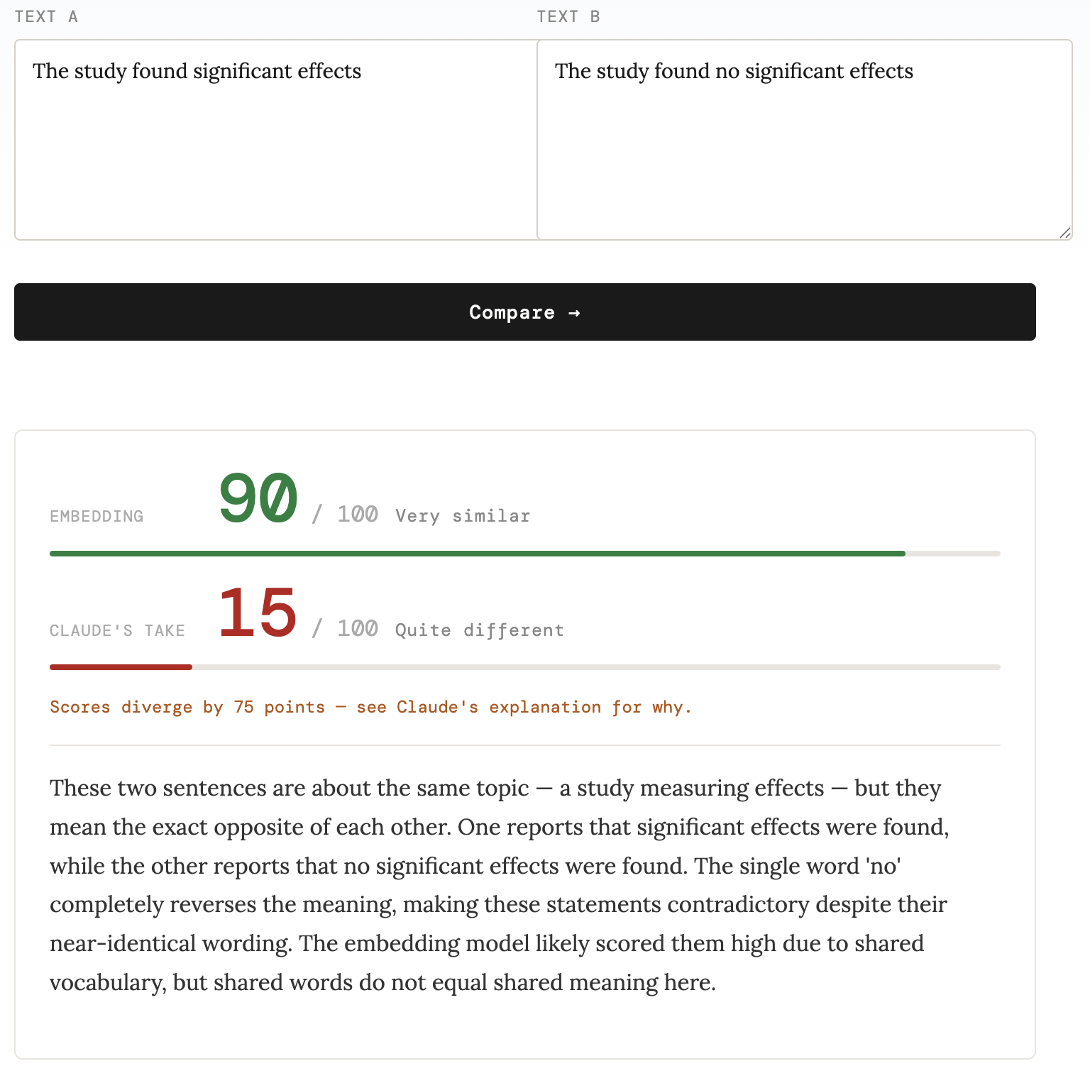
”The study found significant effects” / “The study found no significant effects”	90	15	75 pts
”Think different.” / “Do what you can’t.”	65	55	10 pts

Cross-register paraphrases. Legal contract language and its plain-English restatement — “The licensor shall retain all intellectual property rights not expressly granted herein” vs “The company keeps ownership of everything not specifically handed over” — scored 72 (embedding) vs 88 (Claude). The divergence runs in the opposite direction from the negation cases: Claude scores them higher because it recognizes they’re saying the same thing in different registers. The embedding model is partially pulled toward surface form — the vocabulary overlap is limited, and the formal legal context of “intellectual property” and “licensing” doesn’t map cleanly onto “ownership” and “handed over.”

Antonyms and negations. “The study found significant effects” vs “The study found no significant effects” is the more consequential failure mode. One sentence supports a claim; the other refutes it. They’ll retrieve together on almost any embedding-based system — and in a RAG pipeline surfacing evidence for a claim, that’s not a minor annoyance. The love/hate pair is the intuitive example; this is the one with downstream consequences.

Short texts — a non-divergence worth noting. “Think different.” vs “Do what you can’t.” scored 65 (embedding) and 55 (Claude) — closer than expected, and closer than the other pairs. Both models detected the shared motivational register. The takeaway isn’t that short texts always cause divergence; it’s that when short texts do diverge, the embedding model has almost nothing to work with. Here they happened to share enough tonal signal that both models landed in the same neighborhood.

The embedding model is measuring something real and useful. It’s fast, cheap, scales to billions of documents, and captures genuine semantic relationships that keyword search misses entirely. But it’s measuring a statistical proxy for meaning, learned from distributional patterns in training data — and that proxy breaks down at precisely the cases where meaning is most load-bearing: negation, contradiction, cross-register paraphrase.

Claude’s scores are better calibrated to semantic agreement on those cases — not because it has privileged access to meaning, but for tractable architectural reasons: joint attention over both texts, training on explicit reasoning tasks including entailment and contradiction, autoregressive generation that allows deliberate comparison rather than a single forward pass to a fixed vector. Whether that constitutes “understanding” is genuinely unclear. What’s clear is the behavioral difference, and the class of applications where it matters: contradiction detection, claim verification, legal semantics — anywhere the question is what texts assert rather than what topics they cover.

For those applications, the production answer isn’t to replace embedding retrieval — it’s to add a reranker. A cross-encoder (or an LLM reranker, which is essentially what the Claude step in this tool is doing) re-scores the top-k candidates with full attention over both texts. Fast embedding retrieval gets you the candidates; the reranker catches the negations. The dual-score tool above is a stripped-down version of exactly that pipeline: fast retrieval first, judgment second.

Try it with your own text pairs at /tools/embedding-similarity, or see the embedding space of this blog at /search.